What IS the canonical momentum?

originally posted at https://canmom.tumblr.com/post/115458...

This post is going to try and explain the concepts of Lagrangian mechanics, with minimal derivations and mathematical notation. By the end of it, hopefully you will know what my URL is all about. [note: when this post was written, I was going by 'canonicalmomentum'; it has since been shortened.]

Some mechanicses which happened in the past

In 1687, Isaac Newton became the famousest scientist jerk in Europe by writing a book called Philosophiæ Naturalis Principia Mathematica. The book gave a framework of describing motion of objects that worked just as well for stuff in space as objects on the ground. Physicists spent the next couple of hundred years figuring out all the different things it could be applied to.

(Newton’s mechanics eventually got downgraded to ‘merely a very good approximation’ when quantum mechanics and relativity came along to complicate things in the 1900s.)

In 1788, Joseph-Louise Lagrange found a different way to put Newton’s mechanics together, using some mathematical machinery called Calculus of Variations. This turned out to be a very useful way to look at mechanics, almost always much easier to operate, and also, like, the basis for all theoretical physics today.

We call this Lagrangian mechanics.

What’s the point of a mechanics?

The way we think of it these days is, whatever we’re trying to describe is a physical system. For example, this cool double pendulum.

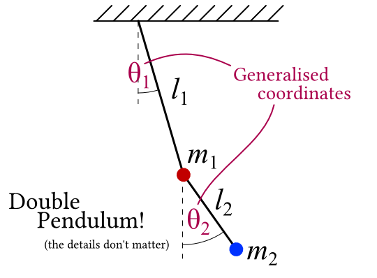
An illustration of a double pendulum as an example of a physical system. The details are not hugely important, but the lengths of the two pendulums, masses, and angles are labelled.

The physical system has a state - “the pieces of the system are arranged this way”. We can describe the state with a list of numbers. The double pendulum might use the angles of the two pendulums. The name for these numbers, in Lagrangian mechanics, is generalised coordinates.

(Why are they “generalised”? When Newton did his mechanics to begin with, everything was thought of as ‘particles’ with a position in 3D space. The coordinates are each particle’s $x$, $y$ and $z$ position. Lagrangian mechanics, on the other hand is cool with any list of numbers can be used to distinguish the different states of the system, so its coordinates are “generalised”.)

Now, we want to know what the system does as time advances. This amounts to knowing the state of the system for every single point in time.

There are lots of possibilities for what a system might do. The double pendulum might swing up and hold itself horizontal forever, for example, or spin wildly. We call each one a path.

Because the generalised coordinates tell apart all the different states of the system, a path amounts to a value of each generalised coordinate at every point in time.

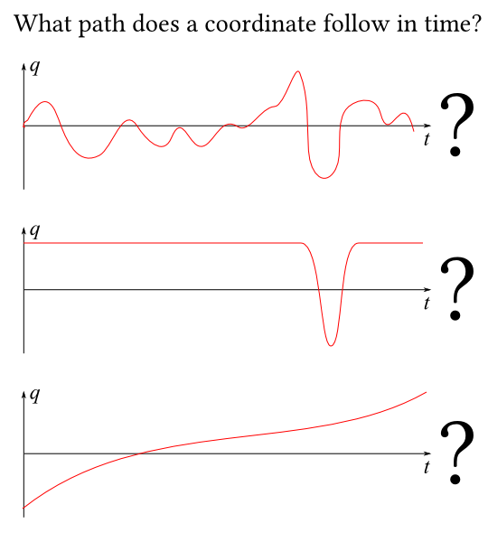
Three example 'paths', as plots of a coordinate q as a function of time t. The first example is a squiggly line, the second q stays the same except for a sudden jump up and down, and the last it smoothly varies.

OK. The point of mechanics is to find out which of the many imaginable paths the system/each coordinate actually takes.

The Action

To achieve this, Lagrangian mechanics says the system has a mathematical object associated with it called the action. It’s almost always written as $S$.

OK, so here’s what you do with the action: you take one of the paths that the system might take, and feed it in; the action then spits out a number. (It’s an object called a functional, to mathematicans: a function from functions to numbers).

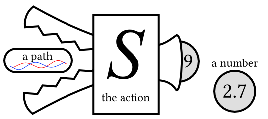
A machine labelled 'the action', S, has large jaws with which a capsule labelled 'a path' enters. On the other side of the machine, grey blobs with 'a number' pop out with various numbers written on them.

So every path the system takes gets a number associated with it by the action.

The actual numbers associated with each path are not actually that useful. Rather, we want to compare ‘nearby’ paths.

We’re looking for a path with a special property: if you add any tiny little extra wiggle to the path, and feed the new path through the action, you get the same number out. We say that the path with this special property is the one the system actually takes.

This is called the principle of stationary action. (It’s sometimes called the “principle of least action”, but since the path we’re interested in is not necessarily the path for which the action is lowest, you shouldn’t call it that.)

But why does it do that

The answer is sort of, because we pick out an action which produces a stationary path corresponding to our system. Which might sound rather circular and pointless.

If you study quantum field theory, you find out the principle of stationary action falls out rather neatly from a calculation called the Path Integral. So you could say that’s “why”, but then you have the question of “why quantum field theory”.

A clearer question is why is it useful to invent an object called the action that does this thing. A couple of reasons:

the general properties actions frequently make it possible to work out the action of a system just by looking at it, and it’s easier to calculate things this way than the Newtonian way.
the action gives us a mathematical object that can be thought of as a ‘complete description of the behaviour of the system’, and conclusions you draw about this object - to do with things like symmetries and conserved quantities, say - are applicable to the system as well.

The Lagrangian

So, OK, let’s crack the action open and look at how it’s made up.

So “inside the action” there’s another object called the Lagrangian, usually written $L$. (As far as I know it got called that by Hamilton, who was a big fan of Lagrange.) The Lagrangian takes a state of the system and a measure of how quickly its changing, and gives you back a number.

The action crawls along the path of the system, applying the Lagrangian at every point in time, and adding up all the numbers.

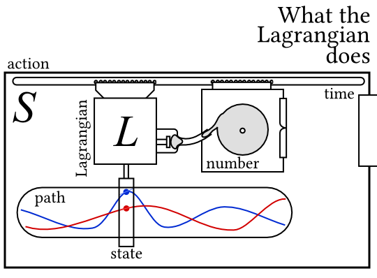
An illustration of the action as a machine. The path sits at the bottom of the machine, and an object called the Lagrangian runs along a rail labelled time at the top, measuring the values on the path at different points. This pushes some grey material onto a blob labelled 'number'. The implication is that the blob's size depends on how the Lagrangian processes the values of the path at various points, and then the blob is ejected.

Mathematically, the action is the integral of the Lagrangian with respect to time. We write that like $$S[q]=\int_{q(t)} L(q,\dot{q},t)\dif t$$

What can you do with a Lagrangian?

Lots and lots of things.

The main thing is that you use the Lagrangian to figure out what the stationary path is.

Using a field of maths called calculus of variations, you can show that the path that stationaryises the action can be found from the Lagrangian by solving a set of differential equations called the Euler-Langrange equations. If you’re curious, they look like $$\frac{\dif}{\dif t}\left(\frac{\partial L}{\partial \dot{q}_i}\right) = \frac{\partial L}{\partial q_i}$$but we won’t go into the details of how they’re derived in this post.

The Euler-Lagrange equations give you the equations of motion of the system. (Newtonian mechanics would also give you the same equations of motion, eventually. From that point on - solving the equations of motion - everything is the same in all your mechanicses).

The Lagrangian has some useful properties. Constraints can be handled easily using the method of Lagrange multipliers, and you can add Lagrangians for components together to get the Lagrangian of a system with multiple parts.

These properties (and probably some others that I’m forgetting) tell us what a Lagrangian made of multiple Newtonian particles looks like, if we know the Lagrangian for a single particle.

Particles and Potentials (the new RPG!)

In the old, Newtonian mechanics, the world is made up of particles, which have a position in space, a number called a mass, and not much else. To determine the particles’ motion, we apply things called forces, which we add up and divide by the mass to give the acceleration of the particle.

Forces have a direction (they’re objects called vectors), and can depend on any number of things, but very commonly they depend on the particle’s position in space. You can have a field which associates a force (number and direction) with every single point in space.

Sometimes, forces have a special property of being conservative. A conservative force has the special property that

depends on where the particle is, but not how fast its going
if you move the particle in a loop, and add up the force times the distance moved at every point around the loop, you get zero

This is great, because now your force can be found from a potential. Instead of associating a vector with every point, the potential is a scalar field which just has a number (no direction) at each point.

This is great for lots of reasons (you can’t get very far in orbital mechanics or electromagnetism without potentials) but for our purposes, it’s handy because we might be able to use it in the Lagrangian.

How Lagrangians are made

So, suppose our particle can travel along a line. The state of the system can be described with only one generalised coordinate - let’s call it $q(t)$. It’s being acted on by a conservative force, with a potential defined along the line which gives the force on the particle.

With this super simple system, the Lagrangian splits into two parts. One of them is $$T=\frac{1}{2}m\dot{q}^2$$which is a quantity which Newtonian mechanics calls the kinetic energy (but we’ll get to energy in a bit!), and the other is just the potential $V(q)$. With these, the Lagrangian looks like $$L=T-V$$and the equations of motion you get are $$m\ddot{q}=-\frac{\dif V}{\dif q}$$exactly the same as Newtonian mechanics.

As it turns out, you can use that idea really generally. When things get relativistic (such as in electromagnetism), it gets squirlier, but if you’re just dealing with rigid bodies acting under gravity and similar situations? $L=T-V$ is all you need.

This is useful because it’s usually a lot easier to work out the kinetic and potential energy of the objects in a situation, then do some differentiation, than to work out the forces on each one. Plus, constraints.

The Canonical Momentum

The canonical momentum in of itself isn’t all that interesting, actually! Though you use it to make Hamiltonian mechanics, and it hints towards Noether’s theorem, so let’s talk about it.

So the Lagrangian depends on the state of the system, and how quickly its changing. To be more specific, for each generalised coordinate $q_i$, you have a ‘generalised velocity’ $\dot{q}_i$ measuring how quickly it is changing in time at this instant. So for example at one particular instant in the double pendulum, one of the angles might be 30 degrees, and the corresponding velocity might be 10 radians per second.

The canonical momenta $p_i$ can be thought of as a measure of how responsive the Lagrangian is to changes in the generalised velocity. Mathematically, it’s the partial differential (keeping time and all the other generalised coordinates and momenta stationary): $$p_i=\frac{\partial L}{\partial \dot{q}_i}$$They’re called momenta by analogy with the quantities linear momentum and angular momentum in Newtonian mechanics. For the example of the particle travelling in a conservative force, the canonical momentum is exactly the same as the linear momentum: $p=m\dot{q}$. And for a rotating body, the canonical momentum is the same as the angular momentum. For a system of particles, the canonical momentum is the sum of the linear momenta.

But be careful! In situations like motion in a magnetic field, the canonical momentum and the linear momentum are different. Which has apparently led to no end of confusion for Actual Physicists with a problem involving a lattice and an electron and somethingorother I can no long remember…

OK a little maths; let’s grab the Euler-Lagrange equations again: $$\frac{\dif}{\dif t} \left(\frac{\partial L}{\partial \dot{q}}\right) = \frac{\partial L}{\partial q_i}$$Hold on. That’s the canonical momentum on the left. So we can write this as $$\frac{\dif p_i}{\dif t} = \frac{\partial L}{\partial q_i}$$Which has an interesting implication: suppose $L$ does not depend on a coordinate directly, but only its velocity. In that case, the equation becomes $$\frac{\dif p_i}{\dif t}=0$$so the canonical momentum corresponding to this coordinate does not change ever, no matter what.

Which is known in Newtonian mechanics as conservation of momentum. So Lagrangian mechanics shows that momentum being conserved is equivalent to the Lagrangian not depending on the absolute positions of the particles…

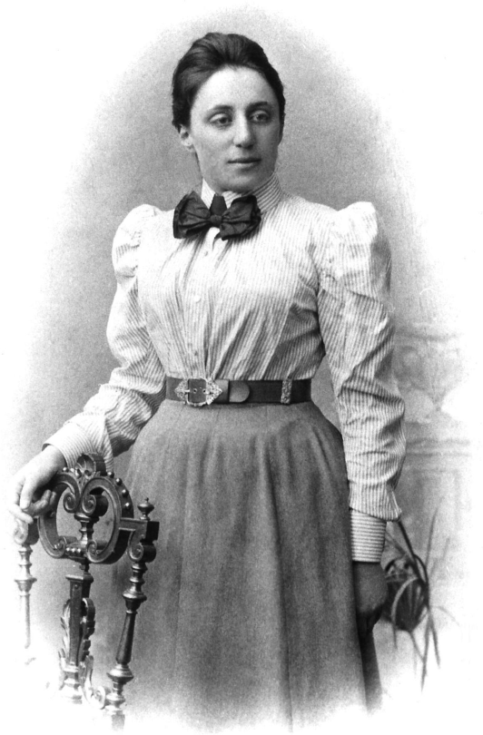
That’s a special case of a very very important theorem invented by Emmy Noether.

The canonical momenta (or in general, the canonical coordinates) are central to a closely related form of mechanics called Hamiltonian mechanics. Hamiltonian mechanics is interesting because it treats the ‘position’ coordinates and ‘momentum’ coordinates almost exactly the same, and because it has features like the ‘Poisson bracket’ which work almost exactly like quantum mechanics. But that can wait for another post.

A greyscale photo of mathematician Emmy Noether. She is wearing a puffy pinstriped shirt, a long grey skirt, and a bow tie.

Coming up next: Noether’s theorem

Lagrangian mechanics may be a useful calculation tool, but the reason it’s important is mainly down to something that Emmy Noether figured out in 1915. This is what I’m talking about when I refer to Lagrangian mechanics forming the basis for all the modern theoretical physics.

[OK, I am a total Noether fangirl. I think I have that it common with most vaguely theoretical physicists (the fan part, not the girl one, sadly). To mathematicians, she’s known for her work in abstract algebra on things like “rings”, but to physicists, it’s all about Noether’s Theorem.]

Noether’s theorem shows that there is a very fundamental relationship between conserved quantities and symmetries of a physical system. I’ll explain what that means in lots more detail in the next post I do, but for the time being, you can read this summary by quasi-normalcy.